The right* way to plot: colorbars
* It really is ... or is it ?
PyCoffee @ Vitacura - 2 June 2016 - fvogt@eso.org
premise:
- colorbars in matplotlib are easy to use and at first it all seems pretty dumb
but as with everything, there is much more to them than meets the eye:
**Colorbars form a magical & untamed Wonderland, where all your wildest dreams can come true !**
http://matplotlib.org/examples/color/colormaps_reference.html
this notebook:
- tips and tricks to tame your colorbars.
utility:
- let your Science rule the colorbar, and not your colorbar rule your Science !
cost:
- From 2 characters to a few lines of code !
gain:
- total control over your colorbars
- accuracy
- elegance
- infinite powers
- ...
take-home message :
- colorbars are fun ... and powerful !
import numpy as np
import matplotlib.pyplot as plt

# Have colormaps separated into categories:
# http://matplotlib.org/examples/color/colormaps_reference.html

cmaps = [('The ONE choice ?',
                            ['viridis', 'inferno', 'plasma', 'magma',
         'Blues', 'BuGn', 'BuPu',
                             'GnBu', 'Greens', 'Greys', 'Oranges', 'OrRd',
                             'PuBu', 'PuBuGn', 'PuRd', 'Purples', 'RdPu',
                             'Reds', 'YlGn', 'YlGnBu', 'YlOrBr', 'YlOrRd',
         'afmhot', 'autumn', 'bone', 'cool',
                             'copper', 'gist_heat', 'gray', 'hot',
                             'pink', 'spring', 'summer', 'winter',
         'BrBG', 'bwr', 'coolwarm', 'PiYG', 'PRGn', 'PuOr',
                             'RdBu', 'RdGy', 'RdYlBu', 'RdYlGn', 'Spectral',
                             'seismic',
         'Accent', 'Dark2', 'Paired', 'Pastel1',
                             'Pastel2', 'Set1', 'Set2', 'Set3',
         'gist_earth', 'terrain', 'ocean', 'gist_stern',
                             'brg', 'CMRmap', 'cubehelix',
                             'gnuplot', 'gnuplot2', 'gist_ncar',
                             'nipy_spectral', 'jet', 'rainbow',
                             'gist_rainbow', 'hsv', 'flag', 'prism'])]

nrows = max(len(cmap_list) for cmap_category, cmap_list in cmaps)
gradient = np.linspace(0, 1, 256)
gradient = np.vstack((gradient, gradient))

def plot_color_gradients(cmap_category, cmap_list):
    fig, axes = plt.subplots(nrows=nrows, figsize=(8,20))
    fig.subplots_adjust(top=0.95, bottom=0.01, left=0.2, right=0.99)
    axes[0].set_title(cmap_category, fontsize=14)

    for ax, name in zip(axes, cmap_list):
        ax.imshow(gradient, aspect='auto', cmap=plt.get_cmap(name))
        pos = list(ax.get_position().bounds)
        x_text = pos[0] - 0.01
        y_text = pos[1] + pos[3]/2.
        fig.text(x_text, y_text, name, va='center', ha='right', fontsize=10)

    # Turn off *all* ticks & spines, not just the ones with colormaps.
    for ax in axes:
        ax.set_axis_off()

fig0 = plt.figure(1, figsize=(20,20))

for cmap_category, cmap_list in cmaps:
    plot_color_gradients(cmap_category, cmap_list)

plt.show()

A) Set the scene
%matplotlib inline
import numpy as np # For creating some fake data
import random

# Ok, let us start by creating some fake data
x,y = np.mgrid[-4:4:0.4,-4:4:0.4]
z = np.sqrt(x**2+y**2)

for i in range(30):

    a = random.choice(range(len(z)))
    b = random.choice(range(len(z)))

    z[a,b] = np.nan

# `randn` generates an array of shape ``(d0, d1, ..., dn)``, filled
# with random floats sampled from a univariate "normal" (Gaussian)
# distribution of mean 0 and variance 1.

# Import the other useful modules
import matplotlib as mpl
import matplotlib.pyplot as plt # Gives access to basic plotting functions
import matplotlib.gridspec as gridspec # GRIDSPEC !
B) A basic example of how most people do things (but shouldn't ?!)
# First, create the figure
plt.close(1)
fig = plt.figure(1, figsize=(12,8))

# The plot itself
plt1 = plt.imshow(z, cmap = 'magma', vmin =0 , vmax = 4, interpolation='nearest')

# Define the limits, labels, ticks as required
plt.grid(True)
plt.ylabel(r'My y label')
plt.xlabel(r'My x label')

plt.colorbar(plt1, label='Colorbar !')

plt.show()

B) The same plot the "proper" way: gridspec !
# First, create the figure
plt.close(1)
fig = plt.figure(1, figsize=(8,8))

# Now, create the gridspec structure, as required
gs = gridspec.GridSpec(1,2, height_ratios=[1], width_ratios=[1,0.05])
gs.update(left=0.05, right=0.95, bottom=0.08, top=0.93, wspace=0.02, hspace=0.03)

ax1 = plt.subplot(gs[0,0])

# The plot itself
plt1 = plt.imshow(z, cmap = 'magma_r', vmin =0 , vmax = 4, interpolation='nearest')

# Define the limits, labels, ticks as required
ax1.grid(True)
ax1.set_ylabel(r'My y label')
ax1.set_xlabel(r'My x label')

# And now the colorbar
# --------------------------------------------------------
cbax = plt.subplot(gs[0,1]) # Place it where it should be.

cb = plt.colorbar(cax = cbax, mappable = plt1, orientation = 'vertical', ticklocation = 'right')
cb.set_label(r'Colorbar !', labelpad=10)

plt.show()

TIP #1: you can invert a named-colorbar by adding _r to its name, e.g.:
magma $\rightarrow$ magma_r
TIP #2: you can place a colorbar horizontaly or vertically.
# First, create the figure
plt.close(1)
fig = plt.figure(1, figsize=(7.6,8))

# Now, create the gridspec structure, as required
gs = gridspec.GridSpec(3,3, height_ratios=[0.05,1,0.05], width_ratios=[0.05,1,0.05])
gs.update(left=0.05, right=0.95, bottom=0.08, top=0.93, wspace=0.02, hspace=0.03)

ax1 = plt.subplot(gs[1,1])

# The plot itself
plt1 = plt.imshow(z, cmap = 'magma_r', vmin =0 , vmax = 4, interpolation='nearest')

# Define the limits, labels, ticks as required
ax1.grid(True)
ax1.set_ylabel(r'')
ax1.set_xlabel(r'')
ax1.set_xticklabels([])
ax1.set_yticklabels([])

# And now the colorbar
# --------------------------------------------------------
# Right
cbax = plt.subplot(gs[1,2]) # Place it where it should be.
cb = plt.colorbar(cax = cbax, mappable = plt1, orientation = 'vertical', ticklocation = 'right')
cb.set_label(r'Colorbar !', labelpad=10)
# Left
cbax = plt.subplot(gs[1,0]) # Place it where it should be.
cb = plt.colorbar(cax = cbax, mappable = plt1, orientation = 'vertical', ticklocation = 'left')
cb.set_label(r'Colorbar !', labelpad=10)
# Top
cbax = plt.subplot(gs[0,1]) # Place it where it should be.
cb = plt.colorbar(cax = cbax, mappable = plt1, orientation = 'horizontal', ticklocation = 'top')
cb.set_label(r'Colorbar !', labelpad=10)
# Top
cbax = plt.subplot(gs[2,1]) # Place it where it should be.
cb = plt.colorbar(cax = cbax, mappable = plt1, orientation = 'horizontal', ticklocation = 'bottom')
cb.set_label(r'Colorbar !', labelpad=10)

plt.show()

C) Discretize colorbars
# To break a colorbar in pieces ... lovely tool !
def cmap_discretize(cmap, N):
    """Return a discrete colormap from the continuous colormap cmap.
    cmap: colormap instance, eg. cm.jet.
    N: number of colors.
    Example
    x = resize(arange(100), (5,100))
    djet = cmap_discretize(cm.jet, 5)
    imshow(x, cmap=djet)
    """
    if type(cmap) == str:
        cmap = mpl.cm.get_cmap(cmap)
    #colors_i = np.concatenate((np.linspace(0, 1., N), (0.,0.,0.,0.)))
    # Fred's update ... dont' start with the colormap edges !
    colors_i = np.concatenate((np.linspace(1./N*0.5, 1-(1./N*0.5), N), (0., 0., 0.)))
    colors_rgba = cmap(colors_i)
    indices = np.linspace(0, 1., N+1)
    cdict = {}
    for ki,key in enumerate(('red','green','blue')):
        cdict[key] = [ (indices[i], colors_rgba[i-1,ki], colors_rgba[i,ki]) for i in xrange(N+1) ]
    # Return colormap object.
    return mpl.colors.LinearSegmentedColormap(cmap.name + "_%d"%N, cdict, 1024)
# Discretize the colorbar into 5 bins
magma_5 = cmap_discretize('magma',5)

# First, create the figure
plt.close(1)
fig = plt.figure(1, figsize=(8,8))

# Now, create the gridspec structure, as required
gs = gridspec.GridSpec(1,2, height_ratios=[1], width_ratios=[1,0.05])
gs.update(left=0.05, right=0.95, bottom=0.08, top=0.93, wspace=0.02, hspace=0.03)

ax1 = plt.subplot(gs[0,0])

# The plot itself
plt1 = plt.imshow(z, cmap = magma_5, vmin =0 , vmax = 4, interpolation='nearest')

# Define the limits, labels, ticks as required
ax1.grid(True)
ax1.set_ylabel(r'My y label')
ax1.set_xlabel(r'My x label')

# And now the colorbar
# --------------------------------------------------------
cbax = plt.subplot(gs[0,1]) # Place it where it should be.

cb = plt.colorbar(cax = cbax, mappable = plt1, orientation = 'vertical', ticklocation = 'right')
cb.set_label(r'Colorbar !', labelpad=10)

plt.show()

D) Improving the colorbar
TIP #3: you can set the colors for NaNs in a colorbar !
TIP #4: Define specific colors for upper and lower limits - to clearly show which point land outside the range !
# Discretize the colorbar into 5 bins
my_Blues = mpl.cm.get_cmap('Blues_r')
my_Blues.set_bad(color=(0.5,0.5,0.5), alpha=1)
my_Blues.set_over(color=(1,0,0), alpha=1)
my_Blues.set_under(color=(0,1,0),alpha=1)

# First, create the figure
plt.close(1)
fig = plt.figure(1, figsize=(8,8))

# Now, create the gridspec structure, as required
gs = gridspec.GridSpec(1,2, height_ratios=[1], width_ratios=[1,0.05])
gs.update(left=0.05, right=0.95, bottom=0.08, top=0.93, wspace=0.02, hspace=0.03)

ax1 = plt.subplot(gs[0,0])

# The plot itself
plt1 = plt.imshow(z, cmap = my_Blues, vmin =1 , vmax = 4, interpolation='nearest')

# Define the limits, labels, ticks as required
ax1.grid(True)
ax1.set_ylabel(r'My y label')
ax1.set_xlabel(r'My x label')

# And now the colorbar
# --------------------------------------------------------
cbax = plt.subplot(gs[0,1]) # Place it where it should be.

cb = plt.colorbar(cax = cbax, mappable = plt1, orientation = 'vertical', ticklocation = 'right')
cb.set_label(r'Colorbar !', labelpad=10)

plt.show()

E) Designing your own colorbar
# Define the inverse-cmap as well
def reverse_colourmap(cdict):
    new_cdict = {}
    for channel in cdict:
        data = []
        for t in cdict[channel]:
            data.append((1. - t[0], t[1], t[2]))

        new_cdict[channel] = data[::-1]
    return new_cdict

# Define the colorbar
cdict_alligator = {
'red'  :  ( (0.00, 0./255, 0./255),
            (0.00, 0./255, 0./255),      (0.2, 20./255., 20./255.),
            (0.40, 46./255., 46./255.),  (0.6, 108./255., 108./255.),
            (0.8, 207./255., 207./255.), (1.00, 255./255.,255./255.),
            (1.00, 255./255, 255./255),),

'green' : ( (0.00, 0./255, 0./255),
            (0.00, 25./255., 25./255.),  (0.2, 85./255., 85./255.),
            (0.4, 139./255., 139./255.), (0.6, 177./255., 177./255.),
            (0.8, 234./255, 234./255),   (1.00, 248./255.,248./255.),
            (1.00, 255./255, 255./255),),

'blue':   ( (0.00, 0./255, 0./255),
            (0.00, 25./255., 25./255.),  (0.2, 81./255., 81./255.),
            (0.4, 87./255., 87./255.),   (0.6, 86./255., 86./255.),
            (0.8, 45./255, 45./255),     (1.00, 215./255.,215./255.),
            (1.00, 255./255, 255./255),),
}

alligator = plt.matplotlib.colors.LinearSegmentedColormap('alligator', cdict_alligator, 1024)
alligator.set_bad(color=(0.5,0.5,0.5), alpha=1)

# And the reverse one
cdict_alligator_r = reverse_colourmap(cdict_alligator)
alligator_r = plt.matplotlib.colors.LinearSegmentedColormap('alligator_r',cdict_alligator_r, 1024)
alligator_r.set_bad(color=(0.5,0.5,0.5), alpha=1)
# First, create the figure
plt.close(1)
fig = plt.figure(1, figsize=(8,8))

# Now, create the gridspec structure, as required
gs = gridspec.GridSpec(1,2, height_ratios=[1], width_ratios=[1,0.05])
gs.update(left=0.05, right=0.95, bottom=0.08, top=0.93, wspace=0.02, hspace=0.03)

ax1 = plt.subplot(gs[0,0])

# The plot itself
plt1 = plt.imshow(z, cmap = alligator_r, vmin =0 , vmax = 4, interpolation='nearest')

# Define the limits, labels, ticks as required
ax1.grid(True)
ax1.set_ylabel(r'My y label')
ax1.set_xlabel(r'My x label')

# And now the colorbar
# --------------------------------------------------------
cbax = plt.subplot(gs[0,1]) # Place it where it should be.

cb = plt.colorbar(cax = cbax, mappable = plt1, orientation = 'vertical', ticklocation = 'right')
cb.set_label(r'Colorbar !', labelpad=10)

plt.show()

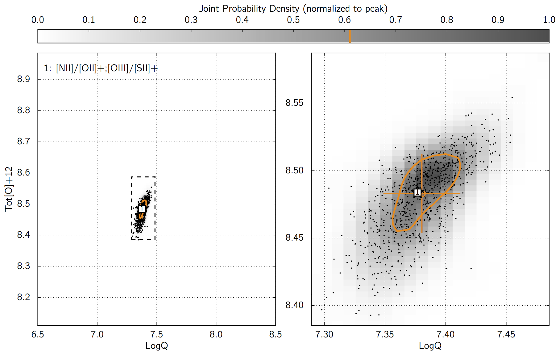
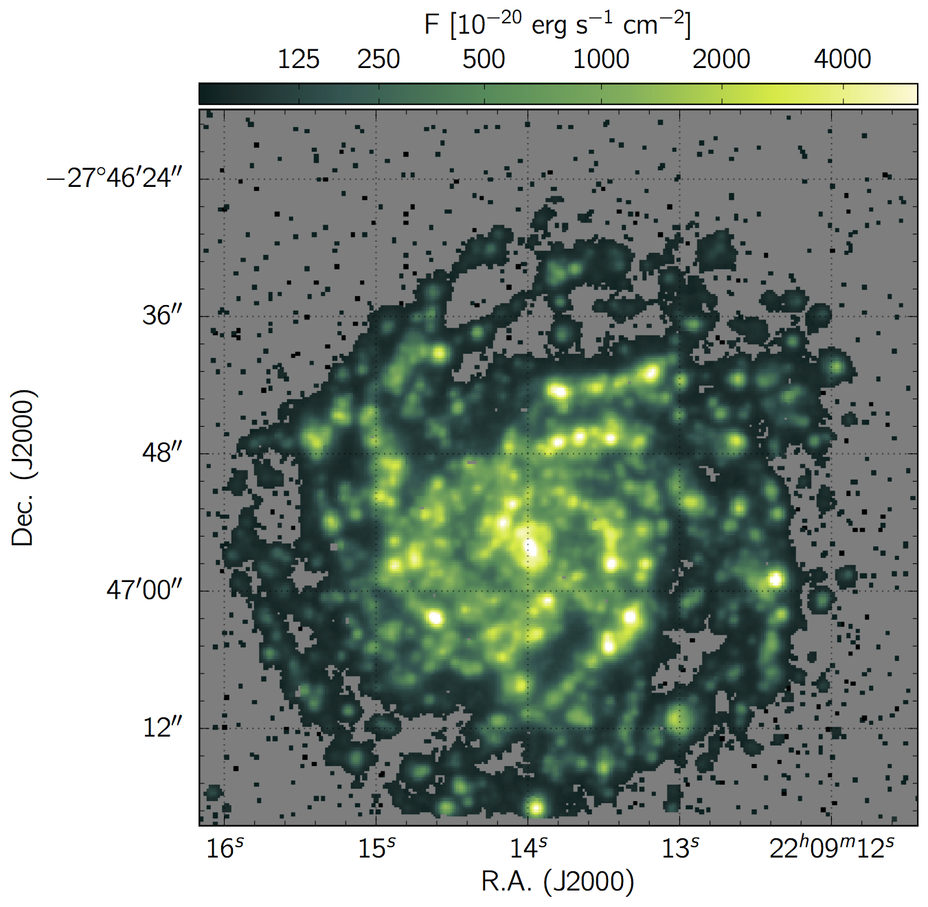
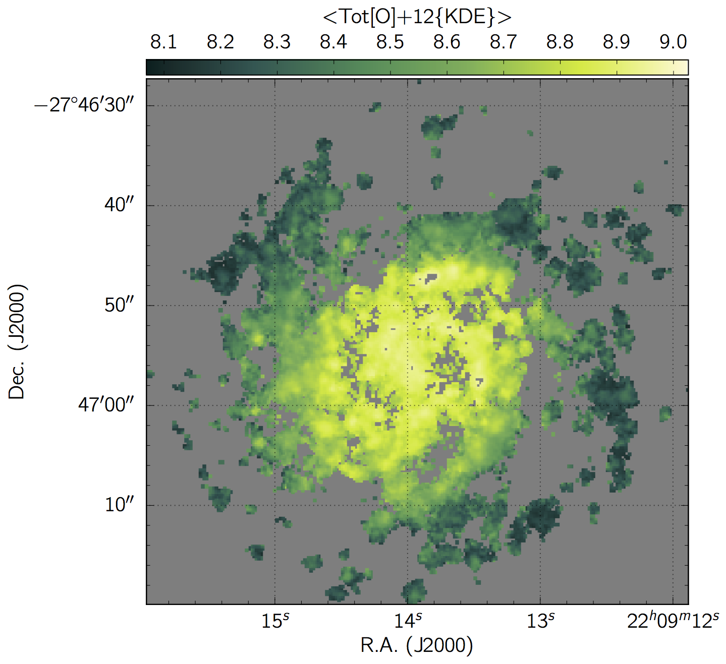
The Alligator in action: http://fpavogt.github.io/brutus/
Another example of a custom colorbar: http://fpavogt.github.io/pyqz/